In the second blog post of our new mini series on Excel Basics, we look at handling large spreadsheets and working with multiple spreadsheets. Sometimes there's such a quantity of information to deal with, it can be hard to know where to start. Luckily, software like Excel can make things a lot easier for you, providing you know how to use it. Read on for some key tips and tricks that will help you on your way to Excel mastery.

Adjusting the View
Excel has some quick methods of zooming in and out of spreadsheets, and dividing up the view of one or several spreadsheets – all of which saves time on searching and scrolling through data.
Use the slider on the right-hand side of the Status bar to zoom in or out.
Splitting Up
If you need to view data that appears in two different parts of the same worksheet, you can split the sheet into two. To do so, select the row or column where you want the divide, click the View tab and press the Split button.
Freezing Panes
Listed data can often be difficult to understand and read if the headings aren’t in view. Go to the View tab and click the Freeze Panes button. Select from the drop-down menu whether you want to keep the top column, first row or both onscreen while moving around a worksheet.
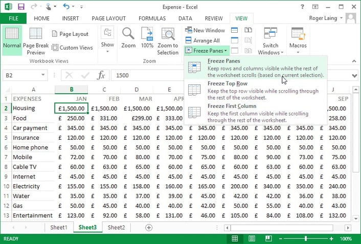
The first row or column in a worksheet can remain visible onscreen when frozen, no matter how far down or across the screen you scroll.
- Hot Tip: Frozen panes can be spotted in a spreadsheet by a thicker line between the cells.
Freeze Multiple Rows and Columns
Select a cell in the spreadsheet where the rows above it and the columns to the left need to remain onscreen, then select the Freeze Panes option as above.
Viewing More Than One Spreadsheet
You can view more than one ‘screen’ at a time in Excel – whether it’s different parts of the same worksheet or completely separate workbooks.
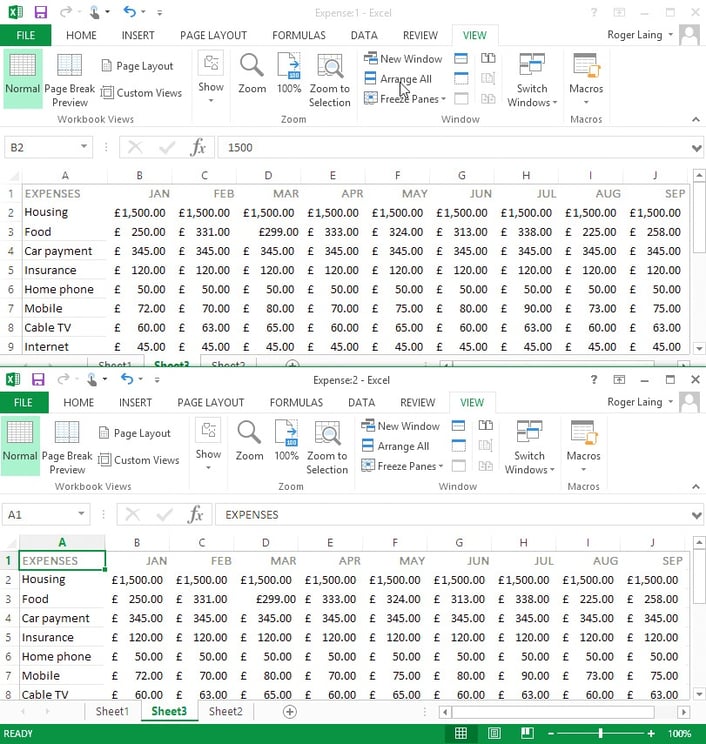
Two or more views of the same worksheet can be set up in Excel by arranging windows.
Make a New Window
If only one spreadsheet is open but you need to look at two different areas of it at once, click the View tab and press the New Window button. A second window showing the spreadsheet will open. Click the Arrange All button and, from the pop-up menu, choose how you want to organize the windows – for example, Vertical puts all the spreadsheets side by side onscreen – then click OK.
Working with More Than One Spreadsheet
Having several spreadsheets displayed onscreen makes it easier to check data and copy information. With the different spreadsheets open, click the Arrange All button, as above, to organize how they are displayed.
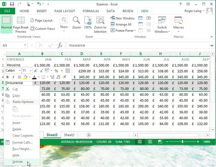
Hidden rows or columns can be revealed by selecting the rows or columns either side, then right-clicking and choosing Unhide.
Hiding Rows and Adding Columns
Rows and columns can be hidden so you see only essential data. Right-click on the column letter or row number and, from the menu that appears, choose Hide. To view it again, select the two columns or rows each side of it, right-click and choose Unhide.
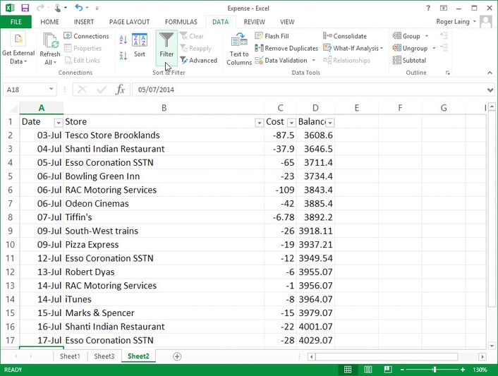
AutoFilter is activated via the Filter button on the Data tab.
This article is a modified version of the text from our new book Every Day Guides Made Easy: Microsoft Excel Basics. To learn more about Excel buy our book from our website, or Amazon.
Links:
- View the first blog in this series 'Navigating Excel on Windows and Mac' by clicking here.
- Check out this incredible Japanese artist who uses Excel to make massive works of art!
- Or click here to read about the guy who built a whole RPG using only Excel. Yes, really.

